Geriatric Nutritional Risk Indexは簡易栄養スクリーニング指標であるが，維持透析患者の死亡率の有意な指標である

　維持透析患者の MIS と死亡率との相関 Zadeh らが報告し，GNRI と MIS との相関の強さは Yamada が報告しておりますが，Yamada の報告では GNRI と透析患者の死亡率との比較はありませんでした．この論文は GNRI と透析患者の死亡率とを直接比較した報告です．

Geriatric Nutritional Risk Indexは簡易栄養スクリーニング指標であるが，維持透析患者の死亡率の有意な指標である

Ikue Kobayashi, Eiji Ishimura, Yoko Kato, Senji Okuno, Tadashi Yamamoto, Tomoyuki Yamakawa, Katsuhito Mori, Masaaki Inaba and Yoshiki Nishizawa

Nephrol Dial Transplant (2010) 25: 3361-3365

要旨

背景

　低栄養は透析患者の一般的合併症である．最近 Geriatric Nutritional Risk Index (GNRI) が透析患者の栄養状態を簡易で正確に評価するツールとして報告されるようになってきた．我々の研究では透析患者の GNRI と死亡率との相関を調査した．

方法

　我々は 490 名の維持透析患者 (60 ± 12 歳，男性 293 名，女性 197 名) の GNRI を調査し，60 ヶ月間に渡って経過を観察した．全死亡の指標を Kaplan-Meyer 法と Cox 比例ハザード法で検証した．

結果

　GNRI は98.0 ± 6.0 であり，有意に年齢および透析期間と負の相関があった．60 ヶ月間の観察期間中 129 名が死亡した．死亡を鑑別する GNRI の陽性尤度比が最大となるカットオフ値は 90 であった．Kaplan-Meyer 法によると GNRI 90 未満の患者 (n = 50) の生存率は 90 以上の患者 (n = 440) と比較して有意に低かった(log-rank検定p < 0.0001)．多変量の Cox 比例ハザード解析ではGNRI が死亡率の有意な指標となることが明らかとなった（年齢，性別，CRP, 糖尿病の存在および透析期間で調整後のハザード比 0.962, 95%CI 0.931 – 0.995, p < 0.05）．

結論

　これらの結果は GNRI が透析患者の死亡率の有意な指標であることを示している．この GNRI の簡易な手法は透析患者の栄養状態を評価する臨床的に有用なマーカーであると考えられる．

キーワード：Geriatric Nutritional Risk Index; haemodialysis; malnutrition; mortality

How to calculate sensitivity, specificity, positive predictive value, negative predictive value, positive likelihood ratio and negative likelihood ratio and their 95 % confidence interval with cross tabulation?

You can calculate 95 % confidence interval of probability as formula below.

$\displaystyle p \pm 1.96 \sqrt{\frac{p(1 - p)}{n}}$

In this article, I’d like to describe how to calculate sensitivity, specificity, positive predictive value (PPV), negative predictive value (NPV), positive likelihood ratio (LR+) and negative likelihood ratio (LR-) and their 95 % confidence interval with cross tabulation.

	TRUE	FALSE	Marginal total
POSITIVE	a	b	a + b
NEGATIVE	c	d	c + d
Marginal total	a + c	b + d	N

Sensitivity, specificity, PPV, NPV, LR+ and LR- and their 95 % confidence interval are shown as following table. ‘Exp()’ means exponential with Napier’s constant and ‘LN()’ means natural logarithmic function, respectively.

	Formula	95% Confidence Interval
Sensitivity	$\displaystyle \frac{a}{a + c}$	$\displaystyle Sensitivity\pm1.96\sqrt{\frac{Sensitivity(1 - Sensitivity)}{a + c}}$
Specificity	$\displaystyle \frac{d}{b + d}$	$\displaystyle Specificity\pm1.96\sqrt{\frac{Specificity(1 - Specificity)}{b + d}}$
PPV	$\displaystyle \frac{a}{a + b}$	$\displaystyle PPV \pm 1.96\sqrt{\frac{PPV(1 - PPV)}{a + b}}$
NPV	$\displaystyle \frac{d}{c + d}$	$\displaystyle NPV \pm 1.96\sqrt{\frac{NPV(1 - NPV)}{c + d}}$
LR+	$\displaystyle \frac{a}{a + c}\bigg/\frac{b}{b + d}$	$\displaystyle Exp \left[LN\left( \frac{Sensitivity}{1 - Specificity}\right)\pm1.96\left(\frac{1 - Sensitivity}{a} + \frac{Specificity}{b}\right) \right]$
LR-	$\displaystyle \frac{c}{a + c}\bigg/\frac{d}{b + d}$	$\displaystyle Exp\left[ LN\left(\frac{1 - Sensitivity}{Specificity}\right) \pm1.96\left( \frac{Sensitivity}{c} + \frac{1 - Specificity}{d} \right)\right]$

感度，特異度，陽性的中率，陰性的中率，陽性尤度比および陰性尤度比とそれぞれの95%信頼区間を計算する

　一般に確率 p の 95 % 信頼区間は下記の式で表現出来ます．

$\displaystyle p \pm 1.96 \sqrt{\frac{p(1 - p)}{n}}$

　今回は四分表から感度，特異度，陽性的中率，陰性的中率，陽性尤度比および陰性尤度比とそれぞれの 95 % 信頼区間を求めます．

	TRUE	FALSE	Marginal total
POSITIVE	a	b	a + b
NEGATIVE	c	d	c + d
Marginal total	a + c	b + d	N

　感度，特異度，陽性的中率，陰性的中率，陽性尤度比および陰性尤度比とそれらの 95 % 信頼区間は下記の通りです．

	Formula	95% Confidence Interval
Sensitivity	$\displaystyle \frac{a}{a + c}$	$\displaystyle Sensitivity\pm1.96\sqrt{\frac{Sensitivity(1 - Sensitivity)}{a + c}}$
Specificity	$\displaystyle \frac{d}{b + d}$	$\displaystyle Specificity\pm1.96\sqrt{\frac{Specificity(1 - Specificity)}{b + d}}$
PPV	$\displaystyle \frac{a}{a + b}$	$\displaystyle PPV \pm 1.96\sqrt{\frac{PPV(1 - PPV)}{a + b}}$
NPV	$\displaystyle \frac{d}{c + d}$	$\displaystyle NPV \pm 1.96\sqrt{\frac{NPV(1 - NPV)}{c + d}}$
LR+	$\displaystyle \frac{a}{a + c}\bigg/\frac{b}{b + d}$	$\displaystyle Exp \left[LN\left( \frac{Sensitivity}{1 - Specificity}\right)\pm1.96\left(\frac{1 - Sensitivity}{a} + \frac{Specificity}{b}\right) \right]$
LR-	$\displaystyle \frac{c}{a + c}\bigg/\frac{d}{b + d}$	$\displaystyle Exp\left[ LN\left(\frac{1 - Sensitivity}{Specificity}\right) \pm1.96\left( \frac{Sensitivity}{c} + \frac{1 - Specificity}{d} \right)\right]$

How to export Excel worksheets to database with SQL statement file.

When you’d like to register Excel worksheets in database, you could ‘BULK INSERT’ txt file into database. In this article, I’d like to explain VBA code that exports Excel worksheets to sql file. It’s assumed that worksheet name is same as table name and first column order is same as table attribute order.

Option Explicit

Sub EXPORT_SQL()
    Dim mySht   As Worksheet
    Dim myAr    As Variant
    Dim i       As Long
    Dim j       As Long
    Dim mySQL   As String
    Dim SQLAr() As String
    Dim myFSO   As Object
    Dim myTS    As Object
    Dim myPath  As String
    Dim n       As Long
    myPath = ThisWorkbook.Path
    For Each mySht In Worksheets
        myAr = mySht.UsedRange.Resize(mySht.UsedRange.Rows.Count - 1).Offset(1)
        ReDim SQLAr(LBound(myAr) To UBound(myAr))
        For i = LBound(myAr) To UBound(myAr)
            For j = LBound(myAr, 2) To UBound(myAr, 2)
                If myAr(i, j) = Empty Then
                    mySQL = mySQL & "NULL, "
                Else
                    mySQL = mySQL & "'" & myAr(i, j) & "', "
                End If
            Next j
            mySQL = "INSERT INTO " & mySht.Name & " VALUES (" & Left(mySQL, Len(mySQL) - 2) & ")"
            SQLAr(i) = mySQL
            mySQL = ""
        Next i
        Set myFSO = CreateObject("Scripting.FileSystemObject")
        Set myTS = myFSO.CreateTextFile(Filename:=myPath & "\" & mySht.Name & ".sql", Overwrite:=True)
        For n = LBound(SQLAr) To UBound(SQLAr)
            myTS.writeline SQLAr(n)
        Next n
        myTS.Close
        Set myFSO = Nothing
        Set myTS = Nothing
    Next mySht
End Sub

EXCELのワークシートをテーブルに挿入するSQLステートメントファイルを作成するVBAコード

　Excel のワークシートをデータベースに登録するにはいくつかの方法があります．txt ファイルを BULK INSERT する方法もありますが，今回はワークシートのセル内容を INSERT するクエリを sql ファイルに書き出す VBA コードを説明します．ワークシート名はテーブル名と同じになっており，ワークシートの1行目はテーブルの属性名と同一の順番になっているとの前提で話を進めます．Excel のファイルと同一場所に sql ファイルがシートの数だけ作成されます．

Option Explicit

Sub EXPORT_SQL()
    Dim mySht   As Worksheet
    Dim myAr    As Variant
    Dim i       As Long
    Dim j       As Long
    Dim mySQL   As String
    Dim SQLAr() As String
    Dim myFSO   As Object
    Dim myTS    As Object
    Dim myPath  As String
    Dim n       As Long
    myPath = ThisWorkbook.Path
    For Each mySht In Worksheets
        myAr = mySht.UsedRange.Resize(mySht.UsedRange.Rows.Count - 1).Offset(1)
        ReDim SQLAr(LBound(myAr) To UBound(myAr))
        For i = LBound(myAr) To UBound(myAr)
            For j = LBound(myAr, 2) To UBound(myAr, 2)
                If myAr(i, j) = Empty Then
                    mySQL = mySQL & "NULL, "
                Else
                    mySQL = mySQL & "'" & myAr(i, j) & "', "
                End If
            Next j
            mySQL = "INSERT INTO " & mySht.Name & " VALUES (" & Left(mySQL, Len(mySQL) - 2) & ")"
            SQLAr(i) = mySQL
            mySQL = ""
        Next i
        Set myFSO = CreateObject("Scripting.FileSystemObject")
        Set myTS = myFSO.CreateTextFile(Filename:=myPath & "\" & mySht.Name & ".sql", Overwrite:=True)
        For n = LBound(SQLAr) To UBound(SQLAr)
            myTS.writeline SQLAr(n)
        Next n
        myTS.Close
        Set myFSO = Nothing
        Set myTS = Nothing
    Next mySht
End Sub

Why probability should be converted to logarithm of odds (logit) in logistic regression analysis?

In logistic regression analysis, probability is converted to odds, p/(1-p), and odds is converted to logarithm. Binomial distribution, either event of interest happens or doesn’t happen, is analysed by multiple regression analysis.

Probability is between 0 and 1. Logarithm of odds (logit) diverges from minus infinity to plus infinity. See charts to understand.

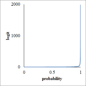
Probability is real between 0 and 1. Take probability horizontal axis and odds vertical axis, respectively. Vertical axis ranges from 0 to infinity, as following chart.

Fig1. probability and logit — Fig1. probability and odds

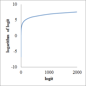
Next, take odds horizontal axis and logarithm of odds vertical axis, respectively. Vertical axis ranges from minus infinity to plus infinity as following chart.

Fig2. logit and logarithm of logit — Fig2. odds and logarithm of odds (logit)

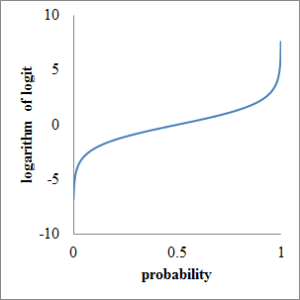
At last, take probability horizontal axis and logit vertical axis, respectively. Although probability ranges only from 0 to 1, logit diverges all real number as following chart.

Fig3. probability and logarithm of logit — Fig3. probability and logit

ロジスティック回帰分析における確率から対数オッズ（ロジット）への変換の意味

　ロジスティック回帰分析においては確率pをオッズ p/(1-p) に変換し，更にオッズの対数（ロジット）を取って回帰分析を行います．この意味を少し考えました．元々は二項分布と言って，ある目的とする事象が起きるか起きないかいずれかの値しか取らない現象を重回帰分析するために考えだされた方法です．世界恐慌直後の米国である疫学調査が行われ，その際に考案された手法だとされています．

　確率 p は 0 から 1 の範囲でしか値を取りません．これをマイナス無限大からプラス無限大の範囲に拡張するのがロジットです．グラフを見たほうが分かりやすいでしょう．

　確率pは 0 以上 1 以下の実数です．横軸を p, 縦軸を $\displaystyle \frac{p}{1-p}$ にグラフを描くと下図のようになります．縦軸のオッズの範囲が 0 以上プラス無限大に拡張しました．

　次に横軸にオッズ，縦軸に対数オッズ（ロジット）を取ってグラフを描くと下図のようになります．対数オッズ（ロジット）の範囲がマイナス無限大からプラス無限大に拡張しました．

　最後に横軸にp, 縦軸に対数オッズ（ロジット）を取ってグラフを描くと下図のようになります．0 から 1 の範囲しか取れなかった確率 p が，対数オッズ（ロジット）に変換されることでマイナス無限大からプラス無限大までの実数に拡張したことが分かります．

Food Composition Tables in the World

In this article, I’d like to introduce food composition tables in the world with on-line web-site. I’m happy if you share more information about other site with me.

Northern Europe
- Finland
- Norway
- Sweden
Western Europe
- Belgium
- Denmark
- Netherlands
- France
- Germany
- Switzerland
- Iceland
- United Kingdom
Eastern Europe
- Czech Republic
- Estonia
- Poland
- Serbia
- Slovakia
Southern Europe
- Greece
- Italy
- Portugal
- Spain
Middle East, Africa
- Bahrain
- Israel
- Middle/Near East
- Mozambique
- South Africa
- Turkey
- West Africa
North America, South America
- Canada
- USA
- Brazil
- Latin America
Oceania
- Australia
- New Zealand
- Pacific Islands
Asia
- China
- Malaysia
- Singapore
- Japan
- Thailand
- Vietnam

Finland

THL

Foods greater than 3400, 54 components. I couldn’t download data file. Rich link forward other country’s food composition tables.

Norway

The Norwegian Food Composition Table

13 food groups, 1305 foods and 36 components. It’s available for download.

Sweden

NFA Food Composition Database

Click “Search nutrient content in food” button below page, click icon of EXCEL and you can download csv file.　Great!

Belgium

NUBEL

1200 foods and 32 components. You need to pay for data.

Denmark

Danish Food Composition Databank

You can download all data with Microsoft Access 2000 or Microsoft EXCEL version 5.0.

Netherlands

NEVO online

Or they would post you EXCEL file with all data if you send form from Request dataset.

France

French food composition table Table Ciqual 2012

You can download from this site csv file or mdb file.

Germany

MRI

Approximately 10,000 foods and 137 components. Read license agreement. Or you can use the Souci Fachmann Kraut Online Database. 800 foods and 260 components. Trial period is 30 days.

Switzerland

Swiss Food Composition Database

13 food groups, 1109 foods and 38 components. Click “Downloads” in left column to download xlsx file.

Iceland

ISGEM

The food composition table of Iceland, provided by MATÍS, seems to be similar to Japanese Food Composition Table. Provided PDF files for each food groups, with protection by password security, respectively. It seems to be 17 food groups.

Or you can purchase at EuroFIR with 15 euros if you visit University College Cork.

United Kingdom

McCance and Widdowson’s The Composition of Foods integrated dataset

Click “Related links” in the middle of page and you can download EXCEL file with 11 MB size and 16 sheets. 13 food groups and 3423 foods.

Czech Republic

Czech Food Composition Database, Version 2.11

13 food groups. You can’t download data file, but reference list is substantial. For example, “McCance and Widdowson’s The Composition of Foods integrated dataset (CoF IDS)” of UK, or “the Ciqual 2012 Table” of France.

Estonia

NutriData – Estonian food composition database

　72 foods and 59 components.

Poland

National Food and Nutrition Institute

Click orange link in right column. 3 steps access level, you need to pay for all 932 foods data and they post EXCEL file in CD-ROM!

Serbia

Department of Nutritional Research (DNR)

You seem to need to log-in and search with Serbia food composition table. But I couldn’t find registration form.

Slovakia

Slovak Food Composition Data Bank (SFCDB)

1419 foods and 52 components.

Greece

COMPOSITION TABLES OF FOODS AND GREEK DISHES

It’s amusing to view Greece food composition table. Instead of citing in the references like Finland, it’s described that they have referred to UK food composition table on site top.

Italy

Tabelle di composizione degli alimenti

Food composition table of Italy has 935 foods, 70 % of them is cited from Europian Institute of Oncology, 30 % is independent survey. GO to Data Search/By Food Group in left column, then you can view all data. Published in 1998 and 2008.

Portugal

TABELA DA COMPOSIÇÃO DE ALIMENTOS

14 food groups and 962 foods. I couldn’t download all data.

Spain

Base de Datos Española de Composición de Alimentos

I have been warned on above page by Google Chrome that security certificate is not trusted. You can enter from “Consulta/Query” on right above the page. 13 food groups, 998 foods and 43 components. I couldn’t download all data.

Bahrain

FOOD COMPOSITON TABLES FOR BAHRAIN

15 food groups and 34 components.

Israel

Ben Gurion University of the Negev

Ben Gurion University of the Negev provides service with simple interface. When you have downloaded “BGU recipe program”, mdb file of Microsoft Access, you could enter recipe in Hebrew and English.

Middle/Near East

food composition tables for the near east

14 food groups, 848 foods and 20 components.

Mozambique

Nutrition research in Mozambique

12 food groups, 410 foods and 35 components. You can download PDF file.

South Africa

South African Medical Research Council

Food composition table of South Africa has tangled link. 4th paragraph of analytical and bibliographic databases, South African Food composition database or Advanced Food composition database is target page. It seems that it had been available for download all data previously, but was not available recently.

Turkey

Turkish Food Composition Database

Turkish food composition database is beta version.

West Africa

Composition of Selected Foods from West Africa

It’s available for download PDF file with 13 food groups and 30 components.

Canada

Canadian Nutrient File (CNF), 2010

Canadian site is intelligent. It’s available for download data file and data structure is clear on the site, it seems to be easy to construct relational database.

USA

the Nutrient Data Laboratory

You can download food composition table of USA as Windows application. If you needed other type file, you could download from USDA National Nutrient Database for Standard Reference with 8.6 MB ASCII file or 21 MB Access file. ASCII file is compressed in zip format with text files and a PDF document, which describes file format and data structure after p26.

Brazil

Tabela de Brasileira de Composição de Alimentos

Food composition table of Brazil provides 1205 foods. It seems that you can’t download data file.

Latin America

Red Latinoamericana de Composición de Alimentos

17 food groups, 443 foods and 24 components. You can’t download data file, but you can view all data on site. This site has links to other Latin America countries.

Australia

NUTTAB 2010

Food composition table of Australia is easy to use and view all data, 19 food groups, 2190 foods and 196 components, with web browser. You can’t download data. You need to register.

New Zealand

New Zealand Food Composition Data for Nutrition Information Panel (NZFCD-NIP)

2700 foods and 7 major components. Windows application is available. It seems that you need to register.

Pacific Islands

The Pacific Islands food composition tables

20 food groups, 882 foods and 22 components. The table is available for download or viewing.

China

China Food Nutrition Network

22 food groups and 14 components. It’s heavy site and mainly written in Chinese.

Malaysia

Malaysian Foods Composition Database; //www.nutriweb.org.my/searchfood.php

Link to food composition table of Malaysia is broken.

Singapore

What’s Eating Singapore

Site of Health Promotion Board is advanced. There are 4 tools on “Health tools” at lower right corner of the page. Energy and Nutrient Composition of Food provides components of each food, Recipe Analysis calculates components of each dish and Food Intake Assessment assess weekly intake from your gender, age and body weight. It’s surprising that they have released smart phone application, BuUuk.

Japan

Report of the Subdivision on Resources The Council for Science and Technology Ministry of Education, Culture, sports, Science and Technology, JAPAN

18 food groups, 1878 foods and 50 components. It’s very difficult to use and convert to database. If you’d like to use immediately, it’s available in my blog, CSV file of the ‘Standard Tables of Food Composition in Japan 2010′.

Thailand

BUREAU OF NUTRITION

In Thailand, they seem to be sensitive to lack of iodine. They have food composition table about 13 food groups and usual 18 components, fatty acid and cholesterol and amino acid.

Vietnam

VIETNAMESE FOOD COMPOSITION TABLE

14 food groups, 526 foods and 86 components.

References:
Food composition databases
National Diet Library of Japan
DTU Food
International food composition table/database directory

世界の食品成分表

オンラインで検索できる世界各国の食品成分表のサイトです．この他にもあると思われますので，ご存知のかたはお知らせいただければ幸いです．

北欧
- フィンランド
- ノルウェー
- スウェーデン
西欧
- ベルギー
- デンマーク
- オランダ
- フランス
- ドイツ
- スイス
- アイスランド
- イギリス
東欧
- チェコ
- エストニア
- ポーランド
- セルビア
- スロバキア
南欧
- ギリシャ
- イタリア
- ポルトガル
- スペイン
中東・アフリカ
- バーレーン
- イスラエル
- 中近東
- モザンビーク
- 南アフリカ
- トルコ
- 西アフリカ
北米・南米
- カナダ
- アメリカ
- ブラジル
- ラテンアメリカ
オセアニア
- オーストラリア
- ニュージーランド
- 太平洋諸島
アジア
- 中国
- マレーシア
- シンガポール
- 日本
- タイ
- ベトナム

フィンランド

THL

フィンランドの食品成分表は3400以上の食品，54種類の栄養素について網羅してあります．日本食品標準成分表は1800種類ですから，数では負けています．残念ながら全データのダウンロードは出来ないようですが，他の国の食品成分表へのリンクが充実しています．

ノルウェー

The Norwegian Food Composition Table

リンクを更新しました．13食品群，1305食品，36成分について提供します．ダウンロード可能です．

スウェーデン

NFA Food Composition Database

スウェーデンの食品成分表は太っ腹です．ページ下部の”Search nutrient content in food”ボタンから入り，ページ右上のEXCELのアイコンをクリックするとcsvファイルがダウンロード出来ます．

ベルギー

NUBEL

1200の食品数，32の栄養素について．全データを入手するには有料のようです．

デンマーク

Danish Food Composition Databank

デンマークのサイトからも全データのダウンロードが可能です．Microsoft Access 2000 形式と，Microsoft Excel v5.0 形式のデータがあります．

オランダ

オランダの食品成分表はNEVO onlineというデータベースから見られます．またはRequest datasetからフォーム送信すると，全データの入ったEXCELのファイルが無料で送付されるようです．但しオランダ語です．

フランス

French food composition table Table Ciqual 2012

フランスの食品成分表はここからcsv形式とmdb形式でダウンロード出来るようになっています．当然ながら，フランス語で書かれています．

ドイツ

MRI

旧西ドイツの食品成分表はフィンランドをはるかに凌ぐ10000近い食品について137栄養素についてデータベース化してあります．生真面目な国民性を反映してか，ここを見る限り自由に利用出来るわけではなさそうで，登録制のようです．ページ最下部からダウンロード出来るPDFにライセンス料金が記載されています．

もうひとつはこちら．800種類の食品の260成分についてのデータベースです．30日間のトライアル期間が設けられています．

スイス

Swiss Food Composition Database

スイスの食品成分表のページの雰囲気は独特です．13の食品群，1109の食品の38の栄養素について提供されます．左カラムに小さく”Downloads“とあり，クリックすると.xlsx形式のファイルをダウンロード出来ます．

アイスランド

ISGEM

アイスランドのMATÍSの食品成分表は日本のそれとよく似ています．食品群ごとにPDFファイルで提供されているところから，プロパティのセキュリティでパスワードロックがかかっていてそのままではコピー出来ないところまで一緒です．提供されているファイル数からは食品群は17に分類されているようです．

もう一つのUniversity College Corkのサイトでは EuroFIRのサイトで買ってねとリンクが貼られているだけです．15ユーロですし，必要な方は購入されてもいいのではないでしょうか．

イギリス

McCance and Widdowson’s The Composition of Foods integrated dataset

イギリスの食品成分表はこのページ中段に”Related links”という章があり，EXCELのファイルでダウンロード出来ます．サイズは11MBもあり16枚のシートから成ります．13の食品群，3423の食品について提供されます．

チェコ

Czech Food Composition Database, Version 2.11

チェコの食品成分表の食品群は13群に分類されています．直接全データをダウンロードはできないのですが，参考文献リストが充実しています．リンクをたどると，イギリスの食品成分表とか，フランスの食品成分表などが出てきます．

エストニア

NutriData – Estonian food composition database

食品数72，59成分について．少ないなあというのが正直な感想です．

ポーランド

National Food and Nutrition Institute

ポーランドの食品成分表は上記ページの右カラムのオレンジ色のFood Composition Data Baseにリンクがあります．3段階のアクセスレベルが設定されていて，932の食品の全データを見るには有料でしかもCD-ROMに収められたEXCELファイルが郵送で送られて来るそうです．

セルビア

Department of Nutritional Research (DNR)

セルビアの食品成分表はログインしてから検索する形式ですが，どうも登録フォームが見当たらず，よく分からないというのが現状です．

スロバキア

Slovak Food Composition Data Bank (SFCDB)

スロバキアの食品成分表は1419の食品の52の成分について提供しています．

ギリシャ

COMPOSITION TABLES OF FOODS AND GREEK DISHES

ギリシャの食品成分表は色々と面白いですね．フィンランドみたいに参考文献の形で引用したとかではなく，イギリスの食品成分表から丸パクりしたと恥ずかしげもなくサイトトップに書いてあります．まあ正直というか，国民性でしょうか．色々想像させられます．3章に分かれており，2章と3章はさすがに自国の伝統料理や日常料理の栄養成分が表記してあります．

イタリア

Tabelle di composizione degli alimenti

イタリアの食品成分表は935種類の食品について調査してありますが，7割がEuropian Institute of Oncologyから引用しており，3割が自前で調査したデータです．全部自前で調べるのではなく，使えるものは使うというスタンスがイタリア人らしいというか何というか．左カラムの/Data Search/By Food Group と進むと全食品のデータが見られます．1998年と2008年の2回刊行されています．

ポルトガル

TABELA DA COMPOSIÇÃO DE ALIMENTOS

ポルトガルの食品成分表は14の食品群，962の食品の42の成分について提供されますが，どうも全データを一括ダウンロードはできないようです．

スペイン

Base de Datos Española de Composición de Alimentos

セキュリティ証明書が信頼出来ないとGoogle Chromeに警告されるページです．こちらから直接入ればよいでしょう．ページ右上の”Consulta/Query”から入れます．13の食品群，998食品の43成分について提供されますが，全データダウンロードは無理のようです．

バーレーン

FOOD COMPOSITON TABLES FOR BAHRAIN

15食品群，34成分について提供します．

イスラエル

Ben Gurion University of the Negev

ベングリオン大学の提供しているサービスです．随分と殺風景なインターフェースですが，ダウンロードしたアクセスのmdbファイルでレシピを入力すると栄養成分が表示されるようになっており，ヘブライ語と英語で入力できるようになっています．

中近東

food composition tables for the near east

14食品群，848食品，20成分について提供します．

モザンビーク

Nutrition research in Mozambique

モザンビークの食品成分表は12食品群，410食品の35成分について提供しています．PDFファイルをダウンロード出来ます．

南アフリカ

South African Medical Research Council

南アフリカの食品成分表はリンクが長く，ややこしいです．このページの4つ目のSouth African Food composition databaseかAdvanced Food composition databaseへリンクを辿るのが良いでしょう．以前は全データが閲覧できたようですが，このフォームからは全データ一括ダウンロードは無理のようです．

トルコ

Turkish Food Composition Database (beta version)

トルコの食品成分表はベータ版です．完成を待ちましょう．

西アフリカ

Composition of Selected Foods from West Africa

西アフリカの食品成分表はPDFファイルでダウンロード可能です．13の食品群，30成分について提供します．

カナダ

Canadian Nutrient File (CNF), 2010

カナダのサイトは充実しています．データファイルを自由にダウンロードでき，かつ各テーブルのデータ構造がサイト上で説明してあるため，これに従ってリレーショナルデータベース化が可能と思われます．

アメリカ

the Nutrient Data Laboratory

アメリカの食品成分表はWindowsアプリケーションをダウンロードさせる形式です．生のデータが欲しい場合はこちらからどうぞ．ASCII形式で8.6MB，Access形式で21MBあります．ダウンロードしたファイルは.zip形式で圧縮されており，フォルダを開くと複数のテキストファイル，pdfファイルが一つあります．pdfはドキュメントであり，p26以降には各ファイルの定義およびデータ構造が記されています．

ブラジル

Tabela de Brasileira de Composição de Alimentos

ブラジルの食品成分表は1205食品の主要な成分を提供します．一括ダウンロードはできないようです．

ラテンアメリカ

Red Latinoamericana de Composición de Alimentos

17の食品群，443の食品の24成分について提供します．ダウンロードは来ませんが全データはブラウザで見られます．中南米各国へのリンクもあります．アルゼンチン，ボリビア，ブラジル，チリ，コロンビア，コスタリカ，メキシコ，ペルー，ウルグアイそれぞれへのリンクがあります．

オーストラリア

NUTTAB 2010

オーストラリアの食品成分表は使い勝手が良く，ブラウザから全データを閲覧出来ます．19食品群，2190食品の196成分について提供します．ただデータの一括ダウンロードは出来ず，登録制になっているようです．

ニュージーランド

ニュージーランドの食品成分表は2700の食品の主要な7成分についてNew Zealand Food Composition Data for Nutrition Information Panel (NZFCD-NIP)が提供しています．ダウンロードできるのはWindows版のアプリケーションです．登録制のようです．

太平洋諸島

The Pacific Islands food composition tables

太平洋諸島の食品成分表は20食品群，882食品の22成分について提供します．ページ上でも閲覧可能で，PDFファイルをダウンロード可能です．

中国

China Food Nutrition Network

22食品群，14成分について提供します．リンクは英文ページですが，実際のデータは主に中国語で書かれています．

マレーシア

Malaysian Foods Composition Database; //www.nutriweb.org.my/searchfood.php

マレーシアのサイトは残念ながらリンク切れです．

シンガポール

シンガポール健康増進委員会のサイトは先進的です．What’s Eating Singaporeというページの右下にHealth Toolsというリンクがあります．Energy and Nutrient Composition of Foodは食品あたりの成分，Recipe Analysisはレシピごとの成分，Food Intake Assessmentでは年齢と性別から一週間の推奨摂取量を計算してくれます．驚くべきことに，BuUukではスマホのアプリまでリリースしています．

日本

文部科学省の資源調査分科会が公表している食品成分表です．18の食品群，1878食品の50成分についてpdfで提供されてるんですが，いかんせん使いにくい．面倒くさい方は，手前味噌ですがこちらからどうぞ．

タイ

BUREAU OF NUTRITION

タイではヨード欠乏に注意を払っていることが伺えます．13食品群，18成分について提供する一般的な食品成分表の他に，脂肪酸とコレステロール，アミノ酸含有量の成分表もあります．

ベトナム

VIETNAMESE FOOD COMPOSITION TABLE

ベトナムの食品成分表は14食品群，526食品の86成分について提供します．

参照：
Food composition databases
国立国会図書館
 DTU Food
International food composition table/database directory

Pearson product-moment correlation coefficient (r) and t-test on it

The index of relation between $x$ and $y$ is correlation coefficient or Pearson product moment correlation coefficient as formula below. Range of correlation coefficient is between -1 and 1.

$\displaystyle r = \frac{\sum_{i=1}^n(x_i-\bar x)(y_i - \bar y)}{\sqrt{\sum_{i=1}^n(x_i - \bar x)^2}\sqrt{\sum_{i=1}^n(y_i - \bar y)^2}}$

$\bar x$ and $\bar y$ are average of $x$ and $y$ , respectively. i is number of sample (incremental variable). n is number of sample.

Correlation coefficient (r) of 2 variables randomly extracted from population follows t-distribution. T-statistics of r is calculated formula as below and follows t-distribution with degree of freedom n-2, n is number of sample. When correlation coefficient of population is $\rho$ , null hypothesis is described that “ $\rho$ = 0″. If t-statistics calculated from number of sample (n) and correlation coefficient (r) is greater than that of significance level ( $\alpha$ ), null hypothesis is rejected.

$\displaystyle t = r\sqrt{\frac{n - 2}{1 - r^2}}$

The test of significance for this important null hypothesis H (ρ = 0) is equivalent to that for the null hypothesis H (β₁ = 0) or H (β₂ = 0). It now follows that if x and y have a joint bivariate normal distribution, then the test for the null hypothesis H (ρ = 0) is obtained by using the fact that if the null hypothesis under test is true, then
$\displaystyle F = \frac{(n-2)Z^2}{XY-Z^2} = \frac{(n-2)r^2}{1-r^2}\vspace{0.1in}\\ X = \sum(x - \bar{x})^2\vspace{0.1in}\\ Y = \sum(y - \bar{y})^2\vspace{0.1in}\\ Z = \sum(x - \bar{x})(y - \bar{y})\vspace{0.1in}\\ r^2 = \frac{Z^2}{XY}$
has the F distribution with 1, n – 2 d.f. An equivalent test of significance for the null hypothesis is obtained by using the fact that if the null hypothesis is true, then
$\displaystyle t = \frac{r\sqrt{n - 2}}{\sqrt{1 - r^2}}$
has “Student’s” distribution. with n – 2 d.f.

For any non-zero null hypothesis about ρ there is no parallelism between the correlation coefficient ρ and the regression coefficients β₁ and β₂. In fact, no exact test of significance is available for testing readily non-zero null hypothesis about ρ. Fisher has given an approximate method for such null hypothesis, but we do not consider this here.

ピアソンの積率相関係数 r とそれに対する t 検定

　 $x$ と $y$ との間の相関の程度を表す指標としてピアソンの積率相関係数 r があり，下記の式で表現します．相関係数 r は -1 から 1 の範囲にあります．

$\displaystyle r = \frac{\sum_{i=1}^n(x_i-\bar x)(y_i - \bar y)}{\sqrt{\sum_{i=1}^n(x_i - \bar x)^2}\sqrt{\sum_{i=1}^n(y_i - \bar y)^2}}$

$\bar x$ and $\bar y$ are average of $x$ and $y$ , respectively. i is number of sample (incremental variable). n is number of sample.

　母集団から無作為に抽出したサンプルの2種類の変数の間の相関係数 r は t 分布に従いますので有意差検定を行うことができます．

　相関係数 r に対する t 統計値は下記の式で求まり，サンプル数 n とすると自由度 n-2 の t 分布に従います．母集団の相関係数を $\rho$ として帰無仮説を『相関係数 $\rho = 0$ である』とします．サンプル数 n, 相関係数 r から計算した t 統計値が，有意水準 $\alpha$ に対応する t 統計値を越えれば帰無仮説を棄却します．

$\displaystyle t = r\sqrt{\frac{n - 2}{1 - r^2}}$

　ピアソンの積率相関係数 r の有意差検定について以前質問をいただきましたが，参考文献を入手しましたので追記します．実は証明など期待していたのですが，期待はずれでした． $\rho$ についての帰無仮説を簡単に検定できる正確な方法は存在しない，と書いてありました．そのような帰無仮説に対して Fisher が近似的な方法を提供していると書かれていましたが，それ以上の記述はありませんでした．以下拙訳です．

　帰無仮説 H (ρ = 0) は次の帰無仮説と同等である．H (β₁ = 0) または H (β₂ = 0)．そこで仮に x, y が共同二変量正規分布を取る場合，仮に検定対象の帰無仮説が真であるとすると，帰無仮説 H (ρ = 0) のための検定が得られる．
$\displaystyle F = \frac{(n-2)Z^2}{XY-Z^2} = \frac{(n-2)r^2}{1-r^2}\vspace{0.1in}\\ X = \sum(x - \bar{x})^2\vspace{0.1in}\\ Y = \sum(y - \bar{y})^2\vspace{0.1in}\\ Z = \sum(x - \bar{x})(y - \bar{y})\vspace{0.1in}\\ r^2 = \frac{Z^2}{XY}$

　上記の F は自由度 n-2 の F 分布に従う．同等の有意差検定として，仮に帰無仮説が真だとすると以下の式は自由度 n-2 の Student’s-t 分布に従う．
$\displaystyle t = \frac{r\sqrt{n - 2}}{\sqrt{1 - r^2}}$

　ρ についてのいかなる帰無仮説でも相関係数 ρ と回帰係数 β₁ および β₂ との間に平行性は存在しない．事実 ρ についての帰無仮説を簡単に検定できる正確な方法は存在しない．そのような帰無仮説に対して Fisher が近似的な方法を提供しているが，ここでは取り扱わない．

How to execute multiple comparison

Student’s t-test would be executed to compare average between two groups. Then if you would like to compare average between 3 or more groups, what do you do? The test needs 2 steps process.

Analysis of variance (ANOVA)
Compare between each 2 groups

1. Analysis of variance

On analysis of variance, null hypothesis is that all groups belong to one population. Therefore, if null hypothesis has been rejected, all groups would not belong to one population.

If all groups belong to one population, the average of all groups, called as grand mean (MG), would be close to average of population. Furthermore, if all groups belong to one population, each average of each groups, for example, M1, M2, M3, would be close to grand mean. However, if any group doesn’t belong to one population, the average of other population would be far from MG. Then we need the indicator that represents how far each average of each groups from grand mean, corrected with number of sample, n. It is called as mean square among groups (MSA).

$\displaystyle MSA = \frac{\sum_{i=1}^k n_i (M_i - MG)^2}{k-1}$

MSA; mean square among groups. n; number of sample in each groups. i; number of group (incremental variable). k; number of groups.

Then calculate variances of each samples, correct with number of each sample and you would take index of variances in samples. It is mean square of error (MSE), average of variance in group.

$\displaystyle MSE = \frac{\sum_{i=1}^k (n_i - 1)V_i}{\sum_{i=1}^{k}(n_i - 1)}$

MSE; mean square of error. n; number of sample in each groups. i; number of group (incremental variable). k; number of groups. V; variance.

$\displaystyle V = \frac{\sum(x - \bar x)^2}{n-1}$

x; each value of samples in each groups. n; number of sample.

F statistics, calculated as ratio MSA to MSE, follows F distribution. When F statistics would be over a value, null hypothesis would be rejected and you could compare average between each groups.

$\displaystyle F=\frac{MSA}{MSE}$

2. Compare between each 2 groups

If null hypothesis would be rejected with ANOVA, you could compare between each groups with following method.

Bonferroni method
Tukey’s HSD
Dunnet’s procedure
Hsu’s MCB tests
Scheffe’s procedure

Bonferroni method may be easy to understand and use. Divided significance level $\alpha$ by k, number of pairs, would be Bonferroni corrected significance level. See following chart.

多重比較するにはまず分散分析を行い，次いで各群間の比較を行う

　2 群間の平均値に差があるかを検定するには Student’s t 検定を行いました．今回は 3 群間の平均値に差があるかを検定する方法を述べます．検定は 2 段階に分けて行います．

分散分析 (ANOVA)
各群間の比較

1. 分散分析 (analysis of variance)

　分散分析では帰無仮説を『全ての群が同一の母集団に属する』とします．これを否定出来れば全ての群が同一母集団には属しないことが言えます．以下その方法を述べます．

　すべての群が同一母集団に属しているなら 3 群全部のサンプル平均値 (grand mean; MG) は母集団の平均値に近くなるはずです．さらにすべての群が同一母集団に属するなら，それぞれの群の平均値 (M1, M2, M3) は MG に近くなるはずです．逆に 3 群が異なる母集団に属するなら M1, M2, M3 は MG から離れた値になります．そこで各群の平均値が総平均値からどれだけ離れているか，それぞれの群のサンプル数 n で補正した指標を下記の式で表現します．これは平均値の群間差の平方和です．

$\displaystyle MSA = \frac{\sum_{i=1}^k n_i (M_i - MG)^2}{k-1}$

MSA; mean square among groups. n; number of sample in each groups. i; number of group (incremental variable). k; number of groups.

　次に各サンプルの分散を求め，各群のサンプル数で補正して 1 サンプルあたりのばらつきの指標とします．これは群内の分散の平均値となります．

$\displaystyle MSE = \frac{\sum_{i=1}^k (n_i - 1)V_i}{\sum_{i=1}^{k}(n_i - 1)}$

MSE; mean square of error. n; number of sample in each groups. i; number of group (incremental variable). k; number of groups. V; variance.

$\displaystyle V = \frac{\sum(x - \bar x)^2}{n-1}$

x; each value of samples in each groups. n; number of sample.

　下記の式のように MSA と MSE の比を取ると， MSA/MSE は F 分布に従います．F の値が一定以上となると帰無仮説は棄却され，全ての群が同一母集団には属しないことが言え，各群間の比較が可能となります．

$\displaystyle F=\frac{MSA}{MSE}$

2. 各群間の比較

　ANOVA の結果，全ての群が同一母集団には属しないことが証明された後に各群間を比較する方法にはいくつかあります．

Bonferroni 法
Tukey 法
Dunnet 法
Hsu’s MCB method
Scheffe’s procedure

　Bonferroni 法が分かりやすいので述べます．有意水準 $\alpha$ を群数 k で除算した $\alpha/k$ を有意水準とする方法です．下図は Bonferroni 法による有意水準を補正した場合としない場合とで有意水準がどう変化するか示したグラフです．

How to estimate 95 % confidence interval of population average from sample average and sample standard deviation?

If you had known average and standard deviation of sample which size is N, you could estimate the range of population average with 95 % probability. In standard normal distribution, sum of area under curve greater than 1.96 and less than – 1.96 is 0.05. There is population average between exception multiplying 1.96 by standard error from average and sum of the multiplied and average, called as 95 % confidence interval (95 % CI).

$\displaystyle 95 \% C.I.= \mu \pm 1.96 SE = \mu \pm 1.96 \frac{SD}{\sqrt N}$

$\mu$ ; Average, SE; standard error, SD; standard deviation

標本平均値と標本標準偏差から母集団の平均値の95％信頼区間を求める

　連続変数においてはサンプルサイズ N の標本の平均値の分布から，95 % の確率で母集団の平均値が含まれる範囲が分かります．標準正規分布においては値が 1.96 以上の曲線下面積と – 1.96 以下の曲線下面積の和は 0.05 となります．つまり標準誤差 SE に 1.96 をかけ，平均値から引いた値から平均値に足した値までの間に真の平均値が含まれます．この範囲を 95 % 信頼区間といいます．

$\displaystyle 95 \% C.I.= \mu \pm 1.96 SE = \mu \pm 1.96 \frac{SD}{\sqrt N}$

$\mu$ ; Average, SE; standard error, SD; standard deviation

Student’s t-test

When you would like to compare two averages between samples, you could use such formulas of Student’s t-test as following chart according to the number and the variances between dependent or independent samples.

Paired t-test as below;

$\displaystyle t = \frac{\bar X_D - \mu_0}{SD/\sqrt{n}} \cdot\cdot\cdot(1)$

Independent two samples t-test with unequal sample sizes and unequal variances, called as Welch’s t-test, as below;

$\displaystyle t = \frac{\bar X_1 - \bar X_2}{SD_p} \cdot\cdot\cdot(2) \vspace{0.2in}\\ SD_p = \sqrt{\frac{SD_1^2}{n_1} + \frac{SD_2^2}{n_2}}$

Independent two samples t-test with equal sample sizes and unequal variances as below;

$\displaystyle t = \frac{\bar X_1 - \bar X_2}{SD_p \sqrt{\frac{2}{n}}} \cdot\cdot\cdot(3) \vspace{0.2in}\\SD_p = \sqrt{\frac{SD_1^2 + SD_2^2}{2}}$

Independent two samples t-test with unequal sample sizes and equal variances as below;

$\displaystyle t = \frac{\bar X_1 - \bar X_2}{SD_p \sqrt{\frac{1}{n_1} + \frac{1}{n_2}}} \cdot\cdot\cdot(4) \vspace{0.2in}\\ SD_p = \sqrt{\frac{(n_1 -1)SD_1^2 + (n_2 - 1)SD_2^2}{n_1 + n_2 - 2}}$

Reference:Student’s t-test

Student t検定

　Student t検定として知られる平均値の検定は下図のフローチャートに従ってどの検定を行うか決めます．

　対応のあるt検定は以下のように求まります．

$\displaystyle t = \frac{\bar X_D - \mu_0}{SD/\sqrt{n}} \cdot\cdot\cdot(1)$

　サンプルサイズが異なり分散も異なる独立した2群の平均値を比較する場合の t 統計値は次式で求まります．Welch検定とも言います．

$\displaystyle t = \frac{\bar X_1 - \bar X_2}{SD_p} \cdot\cdot\cdot(2) \vspace{0.2in}\\ SD_p = \sqrt{\frac{SD_1^2}{n_1} + \frac{SD_2^2}{n_2}}$

　同数かつ等分散の独立した2群の平均値を比べる場合の t 統計値は次式で求まります．

$\displaystyle t = \frac{\bar X_1 - \bar X_2}{SD_p \sqrt{\frac{2}{n}}} \cdot\cdot\cdot(3) \vspace{0.2in}\\SD_p = \sqrt{\frac{SD_1^2 + SD_2^2}{2}}$

　サンプルサイズが異なり等分散の独立した2群の平均値を比較する場合の t 統計値は次式で求まります．

$\displaystyle t = \frac{\bar X_1 - \bar X_2}{SD_p \sqrt{\frac{1}{n_1} + \frac{1}{n_2}}} \cdot\cdot\cdot(4) \vspace{0.2in}\\ SD_p = \sqrt{\frac{(n_1 -1)SD_1^2 + (n_2 - 1)SD_2^2}{n_1 + n_2 - 2}}$

参照：Student’s t-test

t-test on independent groups with unequal variance

Sample average from population which follows normal distribution also follows it. When standard deviation of population is not known, you would have to speculate it with standard deviation of sample. T-statistics follows t-distribution, not normal distribution.

$\displaystyle t = \frac{\bar X - \mu}{SD/\sqrt n} = \frac{\bar X - \mu}{SE} \vspace{0.2in}\\$

SD: standard deviation; SE: standard error

When you would like to compare average values between separate groups with unequal variance, you could calculate t-statistics with formula below;

$\displaystyle t = \frac{(\bar X_2 - \bar X_1)}{SD_p \sqrt{\frac{1}{n_1} + \frac{1}{n_2}}} = \frac{(\bar X_2 - \bar X_1)}{SE}\vspace{0.2in}\\ SD_p = \sqrt{\frac{(n_1 - 1)SD_1^2 + (n_2 -1)SD_2^2}{n_1 + n_2 - 2}}$

$SD_p$ ; pooled SD

When t-statistics is greater than a value, null hypothesis is rejected. In one sided test, when it is greater than the value which area under t-distribution curve is smaller than 0.05, it is statistically significant. In two sided test, when it is greater than the value which area under curve is smaller than 0.025, it is statistically significant. T-statistics follows degree of freedom.

Reference:t-distribution

異分散の独立した2群のt検定

　正規分布に従う母集団からの標本平均値の分布は正規分布に従いますが，母集団の標準偏差 $\sigma$ が未知の場合，サンプルの標準偏差から推測する必要があります．その場合，t 統計値は正規分布ではなく t 分布に従います．

$\displaystyle t = \frac{\bar X - \mu}{SD/\sqrt n} = \frac{\bar X - \mu}{SE} \vspace{0.2in}\\$

　異分散の独立した2群の平均値を比べる場合の t 統計値は次式で求まります．

　t 統計値が t 分布上である値を超えると帰無仮説を棄却します．片側検定の場合，t 分布曲線下の面積が0.05以下になる点を超えれば統計学的有意と判定します．両側検定の場合は0.025以下になる点を超えれば統計学的有意と判定します．統計学的有意となる t 統計値は自由度，つまり標本数により変化します．詳細は下記リンクを参照して下さい．

参照：t分布

How to execute χ-square test with cross tabulation?

You can execute $\chi^2$ test with cross tabulation by such formula as below. In each cells, subtract expected value (E) from observed value (O), square the subtraction, divide the squared by expected value and add them all.

$\displaystyle\chi^2(df)=\sum\frac{(O-E)^2}{E}$

df: degree of freedom

$\chi^2$ statistics follows $\chi^2$ distribution. When degree of freedom is 1, $\chi^2$ statistics is 3.841 if probability is smaller than 0.05 in one sided test, $\chi^2$ is 6.635 if p < 0.01, [latex]\chi^2[/latex] is 10.828 if p < 0.001, respectively. In two-tailed test, [latex]\chi^2[/latex] is 5.024 if p < 0.05, [latex]\chi^2[/latex] is 7.879 if p < 0.01, respectively.

	TRUE	FALSE	Marginal total
POSITIVE	a	b	a + b
NEGATIVE	c	d	c + d
Marginal total	a + c	b + d	N

$\displaystyle \begin{array}{rcl}\chi^2&=&(ad-bc)^2\times\frac{N}{(a+b)(c+d)(a+c)(b+d)}\vspace{0.2in}\\\chi^2(Yates)&=&\left(|ad-bc|-\frac{1}{2}\right)^2\times\frac{N}{(a+b)(c+d)(a+c)(b+d)}\end{array}$

2024年11月
月	火	水	木	金	土	日
				1	2	3
4	5	6	7	8	9	10
11	12	13	14	15	16	17
18	19	20	21	22	23	24
25	26	27	28	29	30