Statistics | Improve Society

How to calculate appropriate sample size in Cox proportional hazard analysis with cross tabulation?

In this article, I’d like to describe how to calculate appropriate sample size in Cox proportional analysis with cross tabulation, a error and b error. a error is called as statistical significance or type 1 error and b error is called as type 2 error, respectively. 1 – b is called as statistical power. a is usually configured at 0.05 (two-tailed) and b is configured at 0.2 (one-sided), respectively. As a result, Z_a/2 is 1.96 and Z_b is 0.84, respectively.

I’d like to assume that S₁ is survival rate of risk group or intervention group and S₀ is survival rate of control group, without risk or intervention. q is ratio of logarithm of them.

$\displaystyle LN(S_1) = Exp(B)LN(S_0)\vspace{0.1in}\\\theta = Exp(B) = \frac{LN(S_1)}{LN(S_0)}$

I’d like to use cross tabulation here. You can replace endpoint with death or failure.

	ENDPOINT	CENSOR	Marginal total
POSITIVE	a	b	a + b
NEGATIVE	c	d	c + d
Marginal total	a + c	b + d	N

$\displaystyle S_1 = \frac{b}{a+b}\vspace{0.1in}\\S_0 = \frac{d}{c+d}$

You can calculate estimated number of death (e) in both group as following formula by Freedman’s approximate calculation.

$\displaystyle e = \left(\frac{\theta+1}{\theta-1}\right)^2(Z_{\alpha/2}+Z_\beta)^2$

You can calculate entry size (n) in each group, as following formula.

$\displaystyle e = n(1-S_0)+n(1-S_1)\vspace{0.1in}\\n = \frac{e}{2 - S_0 - S_1}$

You have to correct entry size with drop-out rate (w) as following formula. Throughout trial, two times of n is needed.

$\displaystyle n = \frac{e}{(2 - S_0 - S_1)(1-w)}$

COX比例ハザードモデルのlog-rank検定に必要なサンプルサイズを四分表から計算する

　COX 比例ハザード解析はリスクの有無や治療介入の有無に対して，生存率や故障率の違いの差を検定する方法です．最終的には四分表に集約可能ですが，解析手段として試験期間にエントリーした症例を，エンドポイント発生までの生存期間を昇順でソートして，エンドポイントが発生するたびに累積生存率を再計算します．

　今回は四分表から計算した生存率の差，aエラー，bエラーから必要なサンプルサイズを計算します．aエラーとは有意確率または第1種の過誤といい，bエラーとは第2種の過誤ともいいます．1 – b のことを検出力といいます．通常ですとa = 0.05（両側），1 – b = 0.8（片側）とすることが多く，その場合 Z_a/2 = 1.96, Z_b = 0.84 とします．当然ながら，リスク群と対照群との生存率の差が小さいほど必要なサンプルサイズは増えます．

　S₁ はリスク群や介入群の生存率，S₀ はリスクなし，介入なしなどいわゆる対照群の生存率とします．q はそれらの対数の比で，追跡終了時点での生存率の比です．

$\displaystyle LN(S_1) = Exp(B)LN(S_0)\vspace{0.1in}\\\theta = Exp(B) = \frac{LN(S_1)}{LN(S_0)}$

　ここで再び四分表が登場します．エンドポイントと打ち切りはそれぞれ死亡と打ち切り，故障と打ち切りなどと読み替え可能です．

	ENDPOINT	CENSOR	Marginal total
POSITIVE	a	b	a + b
NEGATIVE	c	d	c + d
Marginal total	a + c	b + d	N

$\displaystyle S_1 = \frac{b}{a+b}$ $\displaystyle S_0 = \frac{d}{c+d}$

　とすると Freedman による近似計算として両群での期待死亡値 e は下記の式で表現出来ます．

$\displaystyle e = \left(\frac{\theta+1}{\theta-1}\right)^2(Z_{\alpha/2}+Z_\beta)^2$

　n を各群で必要なエントリーサイズとして e をリスク群と対照群の死亡率で割り付けると下記の式で表現出来ます．

$\displaystyle e = n(1-S_0)+n(1-S_1)$

　これを n について解くと下記の式となります．

$\displaystyle n = \frac{e}{2 - S_0 - S_1}$

　脱落率を w とすると補正式は下記のとおりです．試験全体では 2n のサンプルサイズが必要です．

$\displaystyle n = \frac{e}{(2 - S_0 - S_1)(1-w)}$

How to calculate sensitivity, specificity, positive predictive value, negative predictive value, positive likelihood ratio and negative likelihood ratio and their 95 % confidence interval with cross tabulation?

You can calculate 95 % confidence interval of probability as formula below.

$\displaystyle p \pm 1.96 \sqrt{\frac{p(1 - p)}{n}}$

In this article, I’d like to describe how to calculate sensitivity, specificity, positive predictive value (PPV), negative predictive value (NPV), positive likelihood ratio (LR+) and negative likelihood ratio (LR-) and their 95 % confidence interval with cross tabulation.

	TRUE	FALSE	Marginal total
POSITIVE	a	b	a + b
NEGATIVE	c	d	c + d
Marginal total	a + c	b + d	N

Sensitivity, specificity, PPV, NPV, LR+ and LR- and their 95 % confidence interval are shown as following table. ‘Exp()’ means exponential with Napier’s constant and ‘LN()’ means natural logarithmic function, respectively.

	Formula	95% Confidence Interval
Sensitivity	$\displaystyle \frac{a}{a + c}$	$\displaystyle Sensitivity\pm1.96\sqrt{\frac{Sensitivity(1 - Sensitivity)}{a + c}}$
Specificity	$\displaystyle \frac{d}{b + d}$	$\displaystyle Specificity\pm1.96\sqrt{\frac{Specificity(1 - Specificity)}{b + d}}$
PPV	$\displaystyle \frac{a}{a + b}$	$\displaystyle PPV \pm 1.96\sqrt{\frac{PPV(1 - PPV)}{a + b}}$
NPV	$\displaystyle \frac{d}{c + d}$	$\displaystyle NPV \pm 1.96\sqrt{\frac{NPV(1 - NPV)}{c + d}}$
LR+	$\displaystyle \frac{a}{a + c}\bigg/\frac{b}{b + d}$	$\displaystyle Exp \left[LN\left( \frac{Sensitivity}{1 - Specificity}\right)\pm1.96\left(\frac{1 - Sensitivity}{a} + \frac{Specificity}{b}\right) \right]$
LR-	$\displaystyle \frac{c}{a + c}\bigg/\frac{d}{b + d}$	$\displaystyle Exp\left[ LN\left(\frac{1 - Sensitivity}{Specificity}\right) \pm1.96\left( \frac{Sensitivity}{c} + \frac{1 - Specificity}{d} \right)\right]$

感度，特異度，陽性的中率，陰性的中率，陽性尤度比および陰性尤度比とそれぞれの95%信頼区間を計算する

　一般に確率 p の 95 % 信頼区間は下記の式で表現出来ます．

$\displaystyle p \pm 1.96 \sqrt{\frac{p(1 - p)}{n}}$

　今回は四分表から感度，特異度，陽性的中率，陰性的中率，陽性尤度比および陰性尤度比とそれぞれの 95 % 信頼区間を求めます．

	TRUE	FALSE	Marginal total
POSITIVE	a	b	a + b
NEGATIVE	c	d	c + d
Marginal total	a + c	b + d	N

　感度，特異度，陽性的中率，陰性的中率，陽性尤度比および陰性尤度比とそれらの 95 % 信頼区間は下記の通りです．

	Formula	95% Confidence Interval
Sensitivity	$\displaystyle \frac{a}{a + c}$	$\displaystyle Sensitivity\pm1.96\sqrt{\frac{Sensitivity(1 - Sensitivity)}{a + c}}$
Specificity	$\displaystyle \frac{d}{b + d}$	$\displaystyle Specificity\pm1.96\sqrt{\frac{Specificity(1 - Specificity)}{b + d}}$
PPV	$\displaystyle \frac{a}{a + b}$	$\displaystyle PPV \pm 1.96\sqrt{\frac{PPV(1 - PPV)}{a + b}}$
NPV	$\displaystyle \frac{d}{c + d}$	$\displaystyle NPV \pm 1.96\sqrt{\frac{NPV(1 - NPV)}{c + d}}$
LR+	$\displaystyle \frac{a}{a + c}\bigg/\frac{b}{b + d}$	$\displaystyle Exp \left[LN\left( \frac{Sensitivity}{1 - Specificity}\right)\pm1.96\left(\frac{1 - Sensitivity}{a} + \frac{Specificity}{b}\right) \right]$
LR-	$\displaystyle \frac{c}{a + c}\bigg/\frac{d}{b + d}$	$\displaystyle Exp\left[ LN\left(\frac{1 - Sensitivity}{Specificity}\right) \pm1.96\left( \frac{Sensitivity}{c} + \frac{1 - Specificity}{d} \right)\right]$

Why probability should be converted to logarithm of odds (logit) in logistic regression analysis?

In logistic regression analysis, probability is converted to odds, p/(1-p), and odds is converted to logarithm. Binomial distribution, either event of interest happens or doesn’t happen, is analysed by multiple regression analysis.

Probability is between 0 and 1. Logarithm of odds (logit) diverges from minus infinity to plus infinity. See charts to understand.

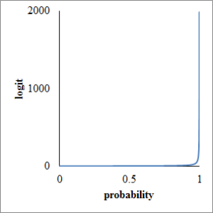
Probability is real between 0 and 1. Take probability horizontal axis and odds vertical axis, respectively. Vertical axis ranges from 0 to infinity, as following chart.

Fig1. probability and logit — Fig1. probability and odds

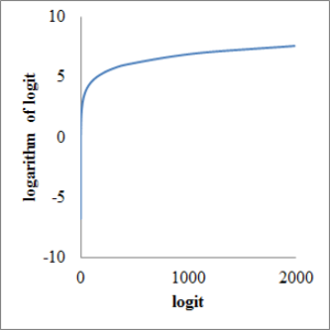
Next, take odds horizontal axis and logarithm of odds vertical axis, respectively. Vertical axis ranges from minus infinity to plus infinity as following chart.

Fig2. logit and logarithm of logit — Fig2. odds and logarithm of odds (logit)

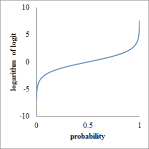
At last, take probability horizontal axis and logit vertical axis, respectively. Although probability ranges only from 0 to 1, logit diverges all real number as following chart.

Fig3. probability and logarithm of logit — Fig3. probability and logit

ロジスティック回帰分析における確率から対数オッズ（ロジット）への変換の意味

　ロジスティック回帰分析においては確率pをオッズ p/(1-p) に変換し，更にオッズの対数（ロジット）を取って回帰分析を行います．この意味を少し考えました．元々は二項分布と言って，ある目的とする事象が起きるか起きないかいずれかの値しか取らない現象を重回帰分析するために考えだされた方法です．世界恐慌直後の米国である疫学調査が行われ，その際に考案された手法だとされています．

　確率 p は 0 から 1 の範囲でしか値を取りません．これをマイナス無限大からプラス無限大の範囲に拡張するのがロジットです．グラフを見たほうが分かりやすいでしょう．

　確率pは 0 以上 1 以下の実数です．横軸を p, 縦軸を $\displaystyle \frac{p}{1-p}$ にグラフを描くと下図のようになります．縦軸のオッズの範囲が 0 以上プラス無限大に拡張しました．

　次に横軸にオッズ，縦軸に対数オッズ（ロジット）を取ってグラフを描くと下図のようになります．対数オッズ（ロジット）の範囲がマイナス無限大からプラス無限大に拡張しました．

　最後に横軸にp, 縦軸に対数オッズ（ロジット）を取ってグラフを描くと下図のようになります．0 から 1 の範囲しか取れなかった確率 p が，対数オッズ（ロジット）に変換されることでマイナス無限大からプラス無限大までの実数に拡張したことが分かります．

Pearson product-moment correlation coefficient (r) and t-test on it

The index of relation between $x$ and $y$ is correlation coefficient or Pearson product moment correlation coefficient as formula below. Range of correlation coefficient is between -1 and 1.

$\displaystyle r = \frac{\sum_{i=1}^n(x_i-\bar x)(y_i - \bar y)}{\sqrt{\sum_{i=1}^n(x_i - \bar x)^2}\sqrt{\sum_{i=1}^n(y_i - \bar y)^2}}$

$\bar x$ and $\bar y$ are average of $x$ and $y$ , respectively. i is number of sample (incremental variable). n is number of sample.

Correlation coefficient (r) of 2 variables randomly extracted from population follows t-distribution. T-statistics of r is calculated formula as below and follows t-distribution with degree of freedom n-2, n is number of sample. When correlation coefficient of population is $\rho$ , null hypothesis is described that “ $\rho$ = 0″. If t-statistics calculated from number of sample (n) and correlation coefficient (r) is greater than that of significance level ( $\alpha$ ), null hypothesis is rejected.

$\displaystyle t = r\sqrt{\frac{n - 2}{1 - r^2}}$

The test of significance for this important null hypothesis H (ρ = 0) is equivalent to that for the null hypothesis H (β₁ = 0) or H (β₂ = 0). It now follows that if x and y have a joint bivariate normal distribution, then the test for the null hypothesis H (ρ = 0) is obtained by using the fact that if the null hypothesis under test is true, then
$\displaystyle F = \frac{(n-2)Z^2}{XY-Z^2} = \frac{(n-2)r^2}{1-r^2}\vspace{0.1in}\\ X = \sum(x - \bar{x})^2\vspace{0.1in}\\ Y = \sum(y - \bar{y})^2\vspace{0.1in}\\ Z = \sum(x - \bar{x})(y - \bar{y})\vspace{0.1in}\\ r^2 = \frac{Z^2}{XY}$
has the F distribution with 1, n – 2 d.f. An equivalent test of significance for the null hypothesis is obtained by using the fact that if the null hypothesis is true, then
$\displaystyle t = \frac{r\sqrt{n - 2}}{\sqrt{1 - r^2}}$
has “Student’s” distribution. with n – 2 d.f.

For any non-zero null hypothesis about ρ there is no parallelism between the correlation coefficient ρ and the regression coefficients β₁ and β₂. In fact, no exact test of significance is available for testing readily non-zero null hypothesis about ρ. Fisher has given an approximate method for such null hypothesis, but we do not consider this here.

ピアソンの積率相関係数 r とそれに対する t 検定

　 $x$ と $y$ との間の相関の程度を表す指標としてピアソンの積率相関係数 r があり，下記の式で表現します．相関係数 r は -1 から 1 の範囲にあります．

$\displaystyle r = \frac{\sum_{i=1}^n(x_i-\bar x)(y_i - \bar y)}{\sqrt{\sum_{i=1}^n(x_i - \bar x)^2}\sqrt{\sum_{i=1}^n(y_i - \bar y)^2}}$

$\bar x$ and $\bar y$ are average of $x$ and $y$ , respectively. i is number of sample (incremental variable). n is number of sample.

　母集団から無作為に抽出したサンプルの2種類の変数の間の相関係数 r は t 分布に従いますので有意差検定を行うことができます．

　相関係数 r に対する t 統計値は下記の式で求まり，サンプル数 n とすると自由度 n-2 の t 分布に従います．母集団の相関係数を $\rho$ として帰無仮説を『相関係数 $\rho = 0$ である』とします．サンプル数 n, 相関係数 r から計算した t 統計値が，有意水準 $\alpha$ に対応する t 統計値を越えれば帰無仮説を棄却します．

$\displaystyle t = r\sqrt{\frac{n - 2}{1 - r^2}}$

　ピアソンの積率相関係数 r の有意差検定について以前質問をいただきましたが，参考文献を入手しましたので追記します．実は証明など期待していたのですが，期待はずれでした． $\rho$ についての帰無仮説を簡単に検定できる正確な方法は存在しない，と書いてありました．そのような帰無仮説に対して Fisher が近似的な方法を提供していると書かれていましたが，それ以上の記述はありませんでした．以下拙訳です．

　帰無仮説 H (ρ = 0) は次の帰無仮説と同等である．H (β₁ = 0) または H (β₂ = 0)．そこで仮に x, y が共同二変量正規分布を取る場合，仮に検定対象の帰無仮説が真であるとすると，帰無仮説 H (ρ = 0) のための検定が得られる．
$\displaystyle F = \frac{(n-2)Z^2}{XY-Z^2} = \frac{(n-2)r^2}{1-r^2}\vspace{0.1in}\\ X = \sum(x - \bar{x})^2\vspace{0.1in}\\ Y = \sum(y - \bar{y})^2\vspace{0.1in}\\ Z = \sum(x - \bar{x})(y - \bar{y})\vspace{0.1in}\\ r^2 = \frac{Z^2}{XY}$

　上記の F は自由度 n-2 の F 分布に従う．同等の有意差検定として，仮に帰無仮説が真だとすると以下の式は自由度 n-2 の Student’s-t 分布に従う．
$\displaystyle t = \frac{r\sqrt{n - 2}}{\sqrt{1 - r^2}}$

　ρ についてのいかなる帰無仮説でも相関係数 ρ と回帰係数 β₁ および β₂ との間に平行性は存在しない．事実 ρ についての帰無仮説を簡単に検定できる正確な方法は存在しない．そのような帰無仮説に対して Fisher が近似的な方法を提供しているが，ここでは取り扱わない．

How to execute multiple comparison

Student’s t-test would be executed to compare average between two groups. Then if you would like to compare average between 3 or more groups, what do you do? The test needs 2 steps process.

Analysis of variance (ANOVA)
Compare between each 2 groups

1. Analysis of variance

On analysis of variance, null hypothesis is that all groups belong to one population. Therefore, if null hypothesis has been rejected, all groups would not belong to one population.

If all groups belong to one population, the average of all groups, called as grand mean (MG), would be close to average of population. Furthermore, if all groups belong to one population, each average of each groups, for example, M1, M2, M3, would be close to grand mean. However, if any group doesn’t belong to one population, the average of other population would be far from MG. Then we need the indicator that represents how far each average of each groups from grand mean, corrected with number of sample, n. It is called as mean square among groups (MSA).

$\displaystyle MSA = \frac{\sum_{i=1}^k n_i (M_i - MG)^2}{k-1}$

MSA; mean square among groups. n; number of sample in each groups. i; number of group (incremental variable). k; number of groups.

Then calculate variances of each samples, correct with number of each sample and you would take index of variances in samples. It is mean square of error (MSE), average of variance in group.

$\displaystyle MSE = \frac{\sum_{i=1}^k (n_i - 1)V_i}{\sum_{i=1}^{k}(n_i - 1)}$

MSE; mean square of error. n; number of sample in each groups. i; number of group (incremental variable). k; number of groups. V; variance.

$\displaystyle V = \frac{\sum(x - \bar x)^2}{n-1}$

x; each value of samples in each groups. n; number of sample.

F statistics, calculated as ratio MSA to MSE, follows F distribution. When F statistics would be over a value, null hypothesis would be rejected and you could compare average between each groups.

$\displaystyle F=\frac{MSA}{MSE}$

2. Compare between each 2 groups

If null hypothesis would be rejected with ANOVA, you could compare between each groups with following method.

Bonferroni method
Tukey’s HSD
Dunnet’s procedure
Hsu’s MCB tests
Scheffe’s procedure

Bonferroni method may be easy to understand and use. Divided significance level $\alpha$ by k, number of pairs, would be Bonferroni corrected significance level. See following chart.

多重比較するにはまず分散分析を行い，次いで各群間の比較を行う

　2 群間の平均値に差があるかを検定するには Student’s t 検定を行いました．今回は 3 群間の平均値に差があるかを検定する方法を述べます．検定は 2 段階に分けて行います．

分散分析 (ANOVA)
各群間の比較

1. 分散分析 (analysis of variance)

　分散分析では帰無仮説を『全ての群が同一の母集団に属する』とします．これを否定出来れば全ての群が同一母集団には属しないことが言えます．以下その方法を述べます．

　すべての群が同一母集団に属しているなら 3 群全部のサンプル平均値 (grand mean; MG) は母集団の平均値に近くなるはずです．さらにすべての群が同一母集団に属するなら，それぞれの群の平均値 (M1, M2, M3) は MG に近くなるはずです．逆に 3 群が異なる母集団に属するなら M1, M2, M3 は MG から離れた値になります．そこで各群の平均値が総平均値からどれだけ離れているか，それぞれの群のサンプル数 n で補正した指標を下記の式で表現します．これは平均値の群間差の平方和です．

$\displaystyle MSA = \frac{\sum_{i=1}^k n_i (M_i - MG)^2}{k-1}$

MSA; mean square among groups. n; number of sample in each groups. i; number of group (incremental variable). k; number of groups.

　次に各サンプルの分散を求め，各群のサンプル数で補正して 1 サンプルあたりのばらつきの指標とします．これは群内の分散の平均値となります．

$\displaystyle MSE = \frac{\sum_{i=1}^k (n_i - 1)V_i}{\sum_{i=1}^{k}(n_i - 1)}$

MSE; mean square of error. n; number of sample in each groups. i; number of group (incremental variable). k; number of groups. V; variance.

$\displaystyle V = \frac{\sum(x - \bar x)^2}{n-1}$

x; each value of samples in each groups. n; number of sample.

　下記の式のように MSA と MSE の比を取ると， MSA/MSE は F 分布に従います．F の値が一定以上となると帰無仮説は棄却され，全ての群が同一母集団には属しないことが言え，各群間の比較が可能となります．

$\displaystyle F=\frac{MSA}{MSE}$

2. 各群間の比較

　ANOVA の結果，全ての群が同一母集団には属しないことが証明された後に各群間を比較する方法にはいくつかあります．

Bonferroni 法
Tukey 法
Dunnet 法
Hsu’s MCB method
Scheffe’s procedure

　Bonferroni 法が分かりやすいので述べます．有意水準 $\alpha$ を群数 k で除算した $\alpha/k$ を有意水準とする方法です．下図は Bonferroni 法による有意水準を補正した場合としない場合とで有意水準がどう変化するか示したグラフです．

How to estimate 95 % confidence interval of population average from sample average and sample standard deviation?

If you had known average and standard deviation of sample which size is N, you could estimate the range of population average with 95 % probability. In standard normal distribution, sum of area under curve greater than 1.96 and less than – 1.96 is 0.05. There is population average between exception multiplying 1.96 by standard error from average and sum of the multiplied and average, called as 95 % confidence interval (95 % CI).

$\displaystyle 95 \% C.I.= \mu \pm 1.96 SE = \mu \pm 1.96 \frac{SD}{\sqrt N}$

$\mu$ ; Average, SE; standard error, SD; standard deviation

標本平均値と標本標準偏差から母集団の平均値の95％信頼区間を求める

　連続変数においてはサンプルサイズ N の標本の平均値の分布から，95 % の確率で母集団の平均値が含まれる範囲が分かります．標準正規分布においては値が 1.96 以上の曲線下面積と – 1.96 以下の曲線下面積の和は 0.05 となります．つまり標準誤差 SE に 1.96 をかけ，平均値から引いた値から平均値に足した値までの間に真の平均値が含まれます．この範囲を 95 % 信頼区間といいます．

$\displaystyle 95 \% C.I.= \mu \pm 1.96 SE = \mu \pm 1.96 \frac{SD}{\sqrt N}$

$\mu$ ; Average, SE; standard error, SD; standard deviation

Student’s t-test

When you would like to compare two averages between samples, you could use such formulas of Student’s t-test as following chart according to the number and the variances between dependent or independent samples.

Paired t-test as below;

$\displaystyle t = \frac{\bar X_D - \mu_0}{SD/\sqrt{n}} \cdot\cdot\cdot(1)$

Independent two samples t-test with unequal sample sizes and unequal variances, called as Welch’s t-test, as below;

$\displaystyle t = \frac{\bar X_1 - \bar X_2}{SD_p} \cdot\cdot\cdot(2) \vspace{0.2in}\\ SD_p = \sqrt{\frac{SD_1^2}{n_1} + \frac{SD_2^2}{n_2}}$

Independent two samples t-test with equal sample sizes and unequal variances as below;

$\displaystyle t = \frac{\bar X_1 - \bar X_2}{SD_p \sqrt{\frac{2}{n}}} \cdot\cdot\cdot(3) \vspace{0.2in}\\SD_p = \sqrt{\frac{SD_1^2 + SD_2^2}{2}}$

Independent two samples t-test with unequal sample sizes and equal variances as below;

$\displaystyle t = \frac{\bar X_1 - \bar X_2}{SD_p \sqrt{\frac{1}{n_1} + \frac{1}{n_2}}} \cdot\cdot\cdot(4) \vspace{0.2in}\\ SD_p = \sqrt{\frac{(n_1 -1)SD_1^2 + (n_2 - 1)SD_2^2}{n_1 + n_2 - 2}}$

Reference:Student’s t-test

Student t検定

　Student t検定として知られる平均値の検定は下図のフローチャートに従ってどの検定を行うか決めます．

　対応のあるt検定は以下のように求まります．

$\displaystyle t = \frac{\bar X_D - \mu_0}{SD/\sqrt{n}} \cdot\cdot\cdot(1)$

　サンプルサイズが異なり分散も異なる独立した2群の平均値を比較する場合の t 統計値は次式で求まります．Welch検定とも言います．

$\displaystyle t = \frac{\bar X_1 - \bar X_2}{SD_p} \cdot\cdot\cdot(2) \vspace{0.2in}\\ SD_p = \sqrt{\frac{SD_1^2}{n_1} + \frac{SD_2^2}{n_2}}$

　同数かつ等分散の独立した2群の平均値を比べる場合の t 統計値は次式で求まります．

$\displaystyle t = \frac{\bar X_1 - \bar X_2}{SD_p \sqrt{\frac{2}{n}}} \cdot\cdot\cdot(3) \vspace{0.2in}\\SD_p = \sqrt{\frac{SD_1^2 + SD_2^2}{2}}$

　サンプルサイズが異なり等分散の独立した2群の平均値を比較する場合の t 統計値は次式で求まります．

$\displaystyle t = \frac{\bar X_1 - \bar X_2}{SD_p \sqrt{\frac{1}{n_1} + \frac{1}{n_2}}} \cdot\cdot\cdot(4) \vspace{0.2in}\\ SD_p = \sqrt{\frac{(n_1 -1)SD_1^2 + (n_2 - 1)SD_2^2}{n_1 + n_2 - 2}}$

参照：Student’s t-test

t-test on independent groups with unequal variance

Sample average from population which follows normal distribution also follows it. When standard deviation of population is not known, you would have to speculate it with standard deviation of sample. T-statistics follows t-distribution, not normal distribution.

$\displaystyle t = \frac{\bar X - \mu}{SD/\sqrt n} = \frac{\bar X - \mu}{SE} \vspace{0.2in}\\$

SD: standard deviation; SE: standard error

When you would like to compare average values between separate groups with unequal variance, you could calculate t-statistics with formula below;

$\displaystyle t = \frac{(\bar X_2 - \bar X_1)}{SD_p \sqrt{\frac{1}{n_1} + \frac{1}{n_2}}} = \frac{(\bar X_2 - \bar X_1)}{SE}\vspace{0.2in}\\ SD_p = \sqrt{\frac{(n_1 - 1)SD_1^2 + (n_2 -1)SD_2^2}{n_1 + n_2 - 2}}$

$SD_p$ ; pooled SD

When t-statistics is greater than a value, null hypothesis is rejected. In one sided test, when it is greater than the value which area under t-distribution curve is smaller than 0.05, it is statistically significant. In two sided test, when it is greater than the value which area under curve is smaller than 0.025, it is statistically significant. T-statistics follows degree of freedom.

Reference:t-distribution

異分散の独立した2群のt検定

　正規分布に従う母集団からの標本平均値の分布は正規分布に従いますが，母集団の標準偏差 $\sigma$ が未知の場合，サンプルの標準偏差から推測する必要があります．その場合，t 統計値は正規分布ではなく t 分布に従います．

$\displaystyle t = \frac{\bar X - \mu}{SD/\sqrt n} = \frac{\bar X - \mu}{SE} \vspace{0.2in}\\$

　異分散の独立した2群の平均値を比べる場合の t 統計値は次式で求まります．

　t 統計値が t 分布上である値を超えると帰無仮説を棄却します．片側検定の場合，t 分布曲線下の面積が0.05以下になる点を超えれば統計学的有意と判定します．両側検定の場合は0.025以下になる点を超えれば統計学的有意と判定します．統計学的有意となる t 統計値は自由度，つまり標本数により変化します．詳細は下記リンクを参照して下さい．

参照：t分布

How to execute χ-square test with cross tabulation?

You can execute $\chi^2$ test with cross tabulation by such formula as below. In each cells, subtract expected value (E) from observed value (O), square the subtraction, divide the squared by expected value and add them all.

$\displaystyle\chi^2(df)=\sum\frac{(O-E)^2}{E}$

df: degree of freedom

$\chi^2$ statistics follows $\chi^2$ distribution. When degree of freedom is 1, $\chi^2$ statistics is 3.841 if probability is smaller than 0.05 in one sided test, $\chi^2$ is 6.635 if p < 0.01, [latex]\chi^2[/latex] is 10.828 if p < 0.001, respectively. In two-tailed test, [latex]\chi^2[/latex] is 5.024 if p < 0.05, [latex]\chi^2[/latex] is 7.879 if p < 0.01, respectively.

	TRUE	FALSE	Marginal total
POSITIVE	a	b	a + b
NEGATIVE	c	d	c + d
Marginal total	a + c	b + d	N

$\displaystyle \begin{array}{rcl}\chi^2&=&(ad-bc)^2\times\frac{N}{(a+b)(c+d)(a+c)(b+d)}\vspace{0.2in}\\\chi^2(Yates)&=&\left(|ad-bc|-\frac{1}{2}\right)^2\times\frac{N}{(a+b)(c+d)(a+c)(b+d)}\end{array}$

四分表（クロス表）からχ二乗検定を行う

　四分表では下記の式でχ二乗統計値を求めるのが一般的ですが，名義変数やアウトカムの取る値が3以上の場合でもχ二乗検定を行うことは可能です．χ二乗統計値とは，全てのセルにおいて観察値 O と期待値 E の差を二乗した値を期待値 E で除し，それらを合計した値のことです．

$\displaystyle\chi^2(df)=\sum\frac{(O-E)^2}{E}$

df: degree of freedom

　四分表（クロス表）が下記のようである場合，χ二乗統計値は次の通りです．χ二乗統計値はχ二乗分布に従い，自由度1の場合，片側検定で p < 0.05 となるχ二乗統計値は 3.841, p < 0.01 だと 6.635, p < 0.001 だと 10.828 です．両側検定で p < 0.05 となるχ二乗統計値は 5.024, P < 0.01 だと 7.879 です．

	TRUE	FALSE	Marginal total
POSITIVE	a	b	a + b
NEGATIVE	c	d	c + d
Marginal total	a + c	b + d	N

When should you execute Fisher exact test, not chi-square test?

You should not execute chi-square test but Fisher exact probability test when gland total of cross tabulation was smaller than 20 or one or greater than one cells had smaller than 5 expected value. In this article, I would like to describe how to solve expected value. Expected value is calculated with marginal total.

We have cross tabulation below;

	TRUE	FALSE	Marginal total
POSITIVE	a	b	a + b
NEGATIVE	c	d	c + d
Marginal total	a + c	b + d	N

Expected value of each cells is below;

	TRUE	FALSE	Marginal total
POSITIVE	(a + b)*(a + c)/N	(a + b)*(b + d)/N	a + b
NEGATIVE	(c + d)*(a + c)/N	(c + d)*(b + d)/N	c + d
Marginal total	a + c	b + d	N

How to calculate Fisher’s exact test with logarithm?

χ二乗検定ではなく Fisher の直接確率検定を行うべき状況とは

　クロス表（四分表）を見て，各セルの期待値が 5 未満の割合が 20 % 以上存在する場合や，総数 N が 20 未満の場合にはχ二乗検定ではなく Fisher の直接確率検定を行うべきであるとされています．この辺り，本来なら Fisher の直接確率検定を行いたいが計算コストが高すぎてχ二乗検定で代用せざるを得なかった経緯があるのではないかと考えます．

　ここでは各セルの期待値を求める方法を述べます．一見して明らかですが，期待値は周辺度数 (marginal total) のみから算出されます．

　下表のようなクロス表があるとします．

	TRUE	FALSE	Marginal total
POSITIVE	a	b	a + b
NEGATIVE	c	d	c + d
Marginal total	a + c	b + d	N

　各セルの期待値は下記の通りです．

	TRUE	FALSE	Marginal total
POSITIVE	(a + b)*(a + c)/N	(a + b)*(b + d)/N	a + b
NEGATIVE	(c + d)*(a + c)/N	(c + d)*(b + d)/N	c + d
Marginal total	a + c	b + d	N

参照記事
対数を用いてFisherの直接確率検定を計算するには

月	火	水	木	金	土	日
				1	2	3
4	5	6	7	8	9	10
11	12	13	14	15	16	17
18	19	20	21	22	23	24
25	26	27	28	29	30